Complex MVA Method Short Circuit Calculation

I. Introduction

This post will present the methodology of MVA Method in performing short circuit calculation. The result will be compared to the Impedance Method of Short-Circuit Calculation and the Per Unit Method later in the article.

The formula used in this example, please refer to Complex MVA Method.

To provide a comparative analysis on the accuracy of each calculation, the example provided in the impedance method will be used in this article just like in the Per Unit Method.

II. Example Calculation

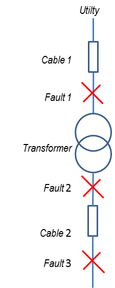
Figure 1 Impedance Method Example — Figure 1 MVA Method Example

From Figure 1, given the parameters below, calculate the 3-phase fault and X/R ratio at Fault 1, Fault 2 and Fault 3:

Utility
Available Fault = 436 MVA
X/R = 15
Cable 1
Length = 1300 m
Unit Resistance = 0.39 ohms/km
Unit Reactance = 0.039 ohms/km
Number of parallel conductors / phase = 1
Transformer
Primary Voltage = 13.8 kV
Secondary Voltage = 0.48 kV
Capacity = 2 MVA
%Z = 5.75%
X/R = 5.662
Cable 2
Length = 500 m
Unit Resistance = 0.048 ohms/km
Unit Reactance = 0.029 ohms/km
Number of parallel conductors / phase = 2

Conversion of Actual Values to MVA

Utility
Available Fault = 436 MVA
X/R = 15
There will be no conversion required for the utility values. The only work here is to break down the MVA into MW and MVAR as

Also, X/R can also be expressed as:

Using eq.1 and eq.2, the MW and MVAR can be calculated.

${I_fault}~=~{MVA~*~1000}/{sqrt{3}~*~kV}~~~~~{right}~eq.5$

Notes:
- Use this online tool to to convert or combine complex quantities connected in series or parallel.
- Refer to this article for the formulas used in the succeeding conversions of actual values into MVA values.

Cable 1
Length = 1300 m
Unit Resistance = 0.39 ohms/km
Unit Reactance = 0.039 ohms/km
Number of parallel conductors / phase = 1

MVA values

MW2 = 371.902279

MVAR2 = 37.1902279

MVA2 = 373.7571647
Transformer
Primary Voltage = 13.8 kV
Secondary Voltage = 0.48 kV
Capacity = 2 MVA
%Z = 5.75%
X/R = 5.662

MVA values

MW3 = 6.049538717

MVAR3 = 34.25248822

MVA3 = 34.7826087

Cable 2
Length = 500 m
Unit Resistance = 0.048 ohms/km
Unit Reactance = 0.029 ohms/km
Number of parallel conductors / phase = 2

MVA values: MW4 = 14.06575517; MVAR4 = 8.498060413; MVA4= 16.43357841

III. Fault Calculations

From the above calculated MVA values, it is now possible to calculate the short-circuit currents at the different fault locations. Please note the MVA values in the following calculations is a complex number as represented by eq.1.

Fault 1 (13.8kV)

MVA~=~1/{1/MVA1+1/MVA2}
MVA~=~1/{({1/{29.00228859+j{435.0343288}})}+(1/{371.902279+j{37.1902279}})}
MVA~=~263.0682965~lt~42.2^o

Calculating the current at Fault1 @ 13.8kV:
$I_{fault1}~=~{263.0682965*1000}/{sqrt{3}*{13.8}}$
$I_{fault1}~=~ 11,005.98 ~{A}$

The X/R value will be:
${X/R}~=~tan(42.2^o)~=~0.91$

Fault 2 (0.48kV)

MVA~=~1/{1/MVA1+1/MVA2+1/MVA3}
MVA~=~1/{({1/{29.00228859+j{435.0343288}})}+(1/{371.902279+j{37.1902279}})+(1/{6.049538717+j{34.25248822}})}
MVA~=~31.4065002~lt~75.79178813^o

Calculating the current at Fault2 @ 0.48kV:
$I_{fault2}~=~{31.4065002*1000}/{sqrt{3}*{0.48}}$
$I_{fault2}~=~ 37,776.15 ~{A}$

The X/R value will be:
${X/R}~=~tan(75.79^o)~=~3.95$

Fault 3 (0.48kV)

MVA~=~1/{1/MVA1+1/MVA2+1/MVA3+1/MVA4}
MVA~=~1/{({1/{29.00228859+j{435.0343288}})}+(1/{371.902279+j{37.1902279}})+(1/{6.049538717+j{34.25248822}})+(1/{14.06575517+j{8.498060413}})}
MVA~=~11.56761387~lt~46.14^o

Calculating the current at Fault3 @ 0.48kV:
$I_{fault2}~=~{11.56761387*1000}/{sqrt{3}*{0.48}}$
$I_{fault2}~=~ 13,913.68 ~{A}$

The X/R value will be:
${X/R}~=~tan(46.14^o)~=~1.04$

IV. Classic MVA Method

The calculation below uses the Classic MVA Method. The MVA value will be a scalar quantity rather than a complex quantity.

Fault 1 (13.8kV)

MVA~=~1/{1/MVA1+1/MVA2}
MVA~=~1/{1/436+1/373.7571647}
MVA~=~201.2432009

Calculating the current at Fault1 @ 13.8kV:
$I_{fault1}~=~{201.2432009*1000}/{sqrt{3}*{13.8}}$
$I_{fault1}~=~ 8,419.41 ~{A}$

Fault 2 (0.48kV)

MVA~=~1/{1/MVA1+1/MVA2+1/MVA3}
MVA~=~1/{({1/{436})+(1/{373.7571647})+(1/{34.7826087})}
MVA~=~29.65677153

Calculating the current at Fault2 @ 0.48kV:
$I_{fault2}~=~{29.65677153*1000}/{sqrt{3}*{0.48}}$
$I_{fault2}~=~ 35,671.55 ~{A}$

Fault 3 (0.48kV)

MVA~=~1/{1/MVA1+1/MVA2+1/MVA3+1/MVA4}
MVA~=~1/{({1/{436})+(1/{373.7571647})+(1/{34.7826087})+(1/{16.43357841})}
MVA~=~ 10.57416316

Calculating the current at Fault3 @ 0.48kV:
$I_{fault3}~=~{10.57416316*1000}/{sqrt{3}*{0.48}}$
$I_{fault3}~=~ 12,718.74~{A}$

V. Impedance Method vs. Per Unit Method vs. MVA Method

The results of the Impedance Method, Per Unit Method and Complex MVA Method are the same hence the accuracy are the same. The Classic MVA Method though has some errors on its results compared to the former.

Comparative Results
Fault	Impedance Method	Per Unit Method	Complex MVA Method	Classic MVA Method
1	11,005.98 A	11,005.98 A	11,005.98 A	8,419.41 A
2	37,776.15 A	37,776.15 A	37,776.15 A	35,671.55 A
3	13,913.68 A	13,913.68 A	13,913.68 A	12,718.74 A